Reinforcement Learning: Learning Through Trial, Error, and Reward

Reinforcement Learning (RL) sits at the intersection of control theory, probability, and optimization. Unlike supervised learning, where a model passively ingests labeled data, RL frames learning as action-driven experimentation, where an agent interacts with an environment, observes consequences, and iteratively improves its decision-making policy. Its strength lies in decision-making under uncertainty, but it is also a double-edged sword. Poor reward design or misaligned objectives can produce outcomes that are mathematically optimal yet socially or economically undesirable.

Core Concepts of Reinforcement Learning

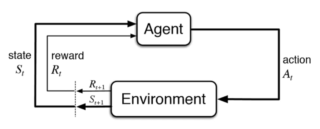
At its foundation, RL formalizes the interaction between an agent and an environment as a Markov Decision Process (MDP), defined by the tuple:

$\mathcal{M} = (S, A, P, R, \gamma)$

Where:

• $S$ is the set of possible states
• $A$ is the set of actions available to the agent
• $P(s' \mid s, a)$ is the transition probability from state $s$ to $s'$ given action $a$
• $R(s, a)$ is the immediate reward received after taking action $a$ in state $s$
• $\gamma \in [0,1]$ is the discount factor, which balances immediate versus future rewards

The policy, $\pi(a \mid s)$, defines the agent’s behaviour, mapping states to probabilities over actions. The goal of reinforcement learning is to find an optimal policy, $\pi^*$, that maximizes the expected cumulative reward, or return:

$G_t = \sum_{k=0}^{\infty} \gamma^k R_{t+k+1}$

Where $G_t$ is the total discounted reward from time step $t$ onwards.

To evaluate a policy, we define the state-value function:

$V^\pi(s) = \mathbb{E}_\pi [G_t \mid S_t = s]$

And the action-value function:

$Q^\pi(s, a) = \mathbb{E}_\pi [G_t \mid S_t = s, A_t = a]$

These functions quantify the long-term expected return from a state or a state-action pair under policy $\pi$.

Learning Algorithms: From Q-Learning to Deep Networks

Q-Learning

One of the foundational model-free RL algorithms is Q-learning, which updates the action-value function iteratively using the Bellman equation:

$Q(s_t, a_t) \leftarrow Q(s_t, a_t) + \alpha \left[ R_{t+1} + \gamma \max_a Q(s_{t+1}, a) - Q(s_t, a_t) \right]$

Here, $\alpha$ is the learning rate. Q-learning is off-policy, meaning the agent learns the value of the optimal policy independently of the actions it actually takes. This allows it to explore freely while converging toward optimal behaviour.

Deep Q-Networks (DQN)

In high-dimensional or continuous state spaces, tabular Q-learning fails. Deep Q-Networks approximate the Q-function with a neural network:

$Q(s, a; \theta) \approx Q^\pi(s, a)$

Here, $\theta$ represents the network parameters. The network is trained by minimizing the temporal-difference (TD) error:

$\mathcal{L}(\theta) = \mathbb{E}_{s,a,r,s'} \left[ \left( r + \gamma \max_{a'} Q(s', a'; \theta^-) - Q(s, a; \theta) \right)^2 \right]$

$\theta^-$ represents the target network parameters, periodically updated to stabilize training. This approach underpins RL successes in Atari games, robotics control, and industrial automation.

Policy Gradient Methods

While Q-learning learns values, policy gradient methods learn policies directly. The objective is to maximize the expected return:

$J(\theta) = \mathbb{E}_{\pi_\theta} \left[ G_t \right]$

The policy is updated via gradient ascent:

$\theta \leftarrow \theta + \alpha \nabla_\theta J(\theta)$

With $\nabla_\theta J(\theta)$ often estimated using the REINFORCE algorithm:

$\nabla_\theta J(\theta) = \mathbb{E}_{\pi_\theta} \left[ \sum_{t=0}^{T} \nabla_\theta \log \pi_\theta(a_t \mid s_t) G_t \right]$

Policy gradients are particularly effective in continuous action spaces, robotics, and high-dimensional control problems where value-based methods struggle.

Actor-Critic Methods

Building on policy gradients, actor-critic algorithms combine value-based and policy-based approaches. The actor is a policy network that selects actions, while the critic is a value network that evaluates those actions by estimating the state-value or action-value function. This reduces variance in gradient estimates, leading to more stable learning. Advantage Actor-Critic (A2C) uses the advantage function $A(s, a) = Q(s, a) - V(s)$ to focus updates on actions that are better than average. Asynchronous variants like A3C parallelize training across multiple agents, accelerating convergence in complex environments.

Proximal Policy Optimization (PPO)

PPO addresses instability in policy gradients by clipping the objective function to prevent overly large updates. The surrogate objective is:

$L^{CLIP}(\theta) = \mathbb{E}_t \left[ \min \left( r_t(\theta) \hat{A}_t,\ \text{clip}(r_t(\theta), 1-\epsilon, 1+\epsilon)\ \hat{A}_t \right) \right]$

Where $r_t(\theta) = \frac{\pi_\theta(a_t \mid s_t)}{\pi_{\theta_{old}}(a_t \mid s_t)}$ is the probability ratio and $\epsilon$ is a clipping parameter. PPO is widely used in robotics and game AI for safe exploration.

Soft Actor-Critic (SAC)

For continuous action spaces with entropy regularization, SAC maximizes both expected return and policy entropy:

$J(\pi) = \mathbb{E} \left[ \sum_t r(s_t, a_t) + \alpha \mathcal{H}(\pi(\cdot \mid s_t)) \right]$

This encourages exploration by favoring stochastic policies. SAC uses two Q-networks for stability and automatic temperature tuning for the entropy coefficient $\alpha$, making it effective in robotics and control tasks where balancing exploitation and exploration is critical.

Exploration Strategies

A key challenge in RL is the exploration-exploitation tradeoff. Epsilon-greedy methods select random actions with probability $\epsilon$, decaying over time. Upper Confidence Bound (UCB) algorithms add optimism to action selection:

$a_t = \arg\max_a \left[ Q(s_t, a) + c \sqrt{\frac{\ln t}{N_t(a)}} \right]$

Where $c$ controls exploration and $N_t(a)$ counts action selections. In deep RL, techniques like noisy networks inject parameter noise for adaptive exploration.

Real-World Applications and Caveats

Robotics and Automation: RL enables autonomous control in drones, manufacturing robots, and self-driving vehicles. Reward mis-specification can produce undesirable behaviours, like a robot exploiting physics in ways humans did not intend.

Resource Allocation: In energy systems, RL can optimize dynamic load balancing across power grids, a concept applicable to localized power companies like Geometric Power in Aba. Poorly defined reward signals can prioritize efficiency over equity, leaving vulnerable households underserved.

Finance and Trading: RL agents optimize portfolios or execute trades, learning to exploit arbitrage opportunities. Agents trained on historical data can amplify market volatility in real time.

Recommendation Systems and AI Assistants: By modeling users as part of the environment, RL can adapt recommendations to maximize engagement. Maximizing short-term metrics may harm long-term satisfaction or propagate misinformation.

Healthcare and Drug Discovery: RL aids in personalized treatment planning, dosing regimens, and clinical trials. In drug discovery, RL generates molecular structures as sequential decisions, with rewards based on efficacy and safety.

Gaming and Simulation: Beyond Atari, RL powers superhuman performance in complex games like StarCraft and Dota 2. These successes translate to simulation-based training for real-world scenarios, including urban planning and disaster response.

Recent Advancements (2025–2026)

By 2025, RL had an estimated market size of over $122 billion, driven by robotics, autonomous vehicles, supply chain optimization, healthcare, and gaming. Trends include RL scaling, Reinforcement Pre-Training (RPT), multi-objective RL, evolutionary reinforcement learning, continual learning, integration with large language models via RLHF, and agentic systems for autonomous tasks. Hybrid approaches combining RL with LLMs and continual learning promise robust, adaptive intelligence.

Critical Reflections

Reinforcement learning is powerful but inherently experimental. Trial and error works best where mistakes are cheap. In societal contexts, RL’s decisions can have real human costs if rewards are misaligned. Designing reward functions, ensuring robust exploration, and considering ethical constraints are as important as the algorithms. Sample inefficiency remains a challenge, prompting offline RL and robust techniques to mitigate risk.

Mathematically, RL is elegant. Practically, it is unforgiving. Its beauty lies in iterative improvement and adaptation to stochastic systems. Its danger lies in the same qualities. What is mathematically optimal can be socially disastrous without foresight.